Summary

Fittings such as elbows, tees, valves and reducers represent a significant component of the pressure loss in most pipe systems. This article details the calculation of pressure losses through pipe fittings and some minor equipment using the 3K method.

Definitions


$D$	:	Internal diameter of pipe
$D_{n}$	:	Nominal diameter of pipe in inches
$K$	:	Resistance Coefficient
$K_{d}$	:	3K method constant
$K_{\infty}$	:	3K method constant
$K_{1}$	:	3K method constant
$Re$	:	Reynolds number

Introduction

The 3K method allows the user to characterise the pressure loss for flow through fittings in a pipe. As the name suggests, three K coefficients are used to characterise the fitting, which when combined with the flow conditions and the pipe diameter may be used to calculate the fitting K value. Once the K value has been determined the head or pressure loss through the fitting may be calculated.

Like the 2K method, the 3K method is an improvement on the K value (excess head) method. While the 2K method improves on the excess head method by characterising the change in pressure loss due to varying Reynolds Number the 3K method further improves the accuracy of the pressure drop prediction by also characterising the change in geometric proportions of a fitting as its size changes. This makes the 3K method particularly accurate for a system with large (greater than DN300/12in) fittings.

For alternative methods of characterising pressure loss for flow through fittings and a discussion of which method is most appropriate please refer to the summary of methods for estimating pressure loss from fittings.

Calculation of K value using the 3K Method

The 3K method is an extension of the 2K method and therefore the Excess Head (K method). As such the 3K method requires the 3K coefficients to be converted into a K value before the fitting pressure drop may be calculated.

Formula for Calculating the K Value from the 3K Method

The K value may be calculated from the 3K coefficients as demonstrated in the equation below.

$K=\frac{K_{1}}{Re}+K_{\infty}\left(1+\frac{K_{d}}{D_{n}^{0.3}}\right)$

As you can see from the equation above the calculation of the K value depends on both the fluid Reynolds number and the size of the fitting.

Table of 3K Coefficients

The table below contains the 3K parameters for a wide range of commonly encountered fittings.

Category	Fitting	Types	$K_{1}$	$K_{\infty}$	$K_{d} (in^{0.3})$	$K_{d} (mm^{0.3})$
Elbow	90° Threaded	Standard Radius (R/D = 1)	800	0.14	4	10.6
Elbow	90° Threaded	Long Radius (R/D = 1.5)	800	0.071	4.2	11.1
Elbow	90° Flanged or Welded	Standard Radius (R/D = 1)	800	0.091	4	10.6
Elbow	90° Flanged or Welded	Long Radius (R/D = 2)	800	0.056	3.9	10.3
Elbow	90° Flanged or Welded	Long Radius (R/D = 4)	800	0.066	3.9	10.3
Elbow	90° Flanged or Welded	Long Radius (R/D = 6)	800	0.075	4.2	11.1
Elbow	90° Mitered	1 weld 90°	1000	0.27	4	10.6
Elbow	90° Mitered	2 welds 45°	800	0.068	4.1	10.8
Elbow	90° Mitered	3 welds 30°	800	0.035	4.2	11.1
Elbow	45° Threaded	Standard Radius (R/D = 1)	500	0.071	4.2	11.1
Elbow	45° Threaded	Long Radius (R/D = 1.5)	500	0.052	4	10.6
Elbow	45° Mitered	1 weld 45°	500	0.086	4	10.6
Elbow	45° Mitered	2 welds 22.5°	500	0.052	4	10.6
Elbow	180° Bend	Threaded, close-return (R/D = 1)	1000	0.23	4	10.6
Elbow	180° Bend	Flanged (R/D = 1)	1000	0.12	4	10.6
Elbow	180° Bend	All types (R/D = 1.5)	1000	0.1	4	10.6
Tee	Through-branch as an Elbow	Threaded (R/D = 1)	500	0.274	4	10.6
Tee	Through-branch as an Elbow	Threaded (R/D = 1.5)	800	0.14	4	10.6
Tee	Through-branch as an Elbow	Flanged (R/D = 1)	800	0.28	4	10.6
Tee	Through-branch as an Elbow	Stub-in branch	1000	0.34	4	10.6
Tee	Run-through	Threaded (R/D = 1)	200	0.091	4	10.6
Tee	Run-through	Flanged (R/D = 1)	150	0.05	4	10.6
Tee	Run-through	Stub-in branch	100	0	0	0
Valve	Angle valve	45°, full line size, $\beta = 1$	950	0.25	4	10.6
Valve	Angle valve	90°, full line size, $\beta = 1$	1000	0.69	4	10.6
Valve	Globe valve	Standard, $\beta = 1$	1500	1.7	3.6	9.5
Valve	Plug valve	Branch flow	500	0.41	4	10.6
Valve	Plug valve	Straight through	300	0.084	3.9	10.3
Valve	Plug valve	Three-way (flow through)	300	0.14	4	10.6
Valve	Gate valve	Standard, $\beta = 1$	300	0.037	3.9	10.3
Valve	Ball valve	Standard, $\beta = 1$	300	0.017	3.5	9.2
Valve	Diaphragm	Dam type	1000	0.69	4.9	12.9
Valve	Swing check valve	$V_{\min} = 35[\rho (\text{lb}_{\text{m}}/\text{ft}^{3})]^{-1/2}$	1500	0.46	4	10.6
Valve	Lift check valve	$V_{\min} = 40[\rho (\text{lb}_{\text{m}}/\text{ft}^{3})]^{-1/2}$	2000	2.85	3.8	10

Example Calculation of Pressure Loss using 3K-values

Overview

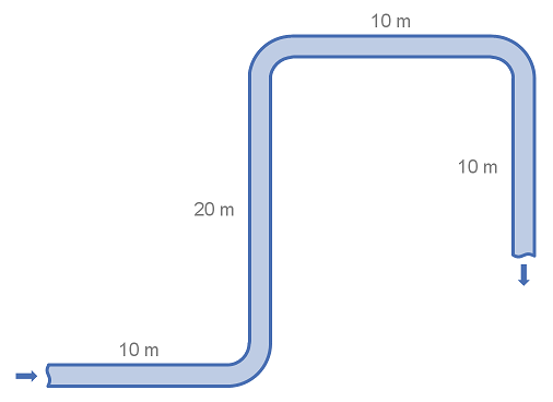
This example demonstrates how to use the 3K method to calculate the head loss through simple pipe and fitting arrangement. The example uses water in system of standard weight carbon steel pipe. Note that for this example we consider a flat system, with no elevation changes.

Equivalent Length Example

System details

Item	Value
Pipe Size	DN100 (4")
Pipe Diameter (Nominal)	4"
Pipe Internal Diameter	102.3 mm
Pipe Length	50 m
Fittings	3 × 90° long radius (R/D = 2) flanged elbows
Fluid Velocity	3 m/s
Fluid Density	1000 kg/m^{3}
Reynolds Number	306,900
Friction Factor	0.018
Gravitational Acceleration	9.81 m/s^{2}

Calculation

Using the table of fittings and 3K-values above we find that the excess head or K-value for the 90° elbow.

$\begin{aligned} K &= \frac{K_{1}}{Re}+K_{\infty}\left(1+\frac{K_{d}}{D_{n}^{0.3}}\right) \\ K &= \frac{800}{306,900}+0.056 \left(1+\frac{3.9}{4^{0.3}}\right) \\ K &= 0.203 \end{aligned}$

With this we can calculate the head loss for a single elbow.

$\begin{aligned} h_{L} &= K \frac{V^{2}}{2g} \\ h_{L} &= 0.203 \frac {3^{2}}{2 \times 9.81} \\ h_{L} &= 0.0931 \text{ m} \end{aligned}$

Using the equation for head loss in pipe, we can calculate the loss through the straight piping:

$\begin{aligned} h_{P} &= f \frac{L}{D} \frac{V^{2}}{2g} \\ h_{P} &= 0.018 \frac{50}{102.3/1000} \frac{3^{2}}{2 \times 9.81} \\ h_{P} &= 4.03 \text{ m} \end{aligned}$

The total head loss for the system is the addition of the head loss from the pipe and the fittings.

$\begin{aligned} h_{T} &= h_{P} + 3 \times h_{L} \\ h_{T} &= 4.03 + 3 \times 0.0931 \\ h_{T} &= 4.30 \text{ m} \end{aligned}$

In the above example we first calculated the head loss for a single fitting and then multiplied by the number of fittings. It is also correct to add or multiply the K-values of fittings and then convert to a pressure or head loss. This is useful when there are many fittings of several types. However the 3K values must be converted to single K values for each fitting type individually.

Pressure Loss from Fittings - 3K Method