Summary
This article provides methods to calculate the K-value (Resistance Coefficient) for determining the pressure loss cause by changes in the area of a fluid flow path. These types of pressure drops are highly dependent on the geometry and are not usually covered in simple pressure loss estimation schemes (such as a single k-value, equivalent length etc.)
Definitions
| : | Internal diameter of pipe | |
| : | Diameter of the upstream pipe | |
| : | Diameter of the downstream pipe | |
| : | Darcy friction factor | |
| : | Resistance Coefficient | |
| : | Length as indicated | |
| : | Reynolds number in upstream pipe | |
| : | Average velocity | |
| : | Angle indicated in degrees |
Introduction
Changes in flow path area where a fluid may be accelerated and/or decelerated such as restriction orifices, pipe reducers and expanders, venturi meters etc. will result in some pressure lost. There are two components to the pressure loss/gain through an area change, the permanent pressure loss and the change due to acceleration. As the name suggests the permanent pressure loss is not recoverable, and like the pressure loss through ordinary fittings such as a pipe elbow, it is lost to friction, eddies, and noise. Pressure changes due to acceleration are reversible, for example in a system where the pipe area decreases, some potential energy in the form of pressure is converted to kinetic energy as the fluid is accelerated in the smaller pipe, reducing the fluid pressure in this pipe. In a perfect system if the fluid then entered a larger pipe and decelerated the kinetic energy of the fluid would be converted back into pressure.
The degree of permanent pressure lost through a pipe size change is dependent on the geometry of the size change. Generally the more abrupt the change the higher the losses, while more gradual changes result in much lower pressure drops. Section 3 presented the equations required to determine the pressure loss through various geometries in terms of K values.
The K value may be converted into head loss through multiplication with the fluid velocity head as shown in the equation below.
Some methods require the friction factor to be known of the pipe. For full details of the method of calculating the friction factor see pressure loss from pipe.
Calculation of K-values for Pipe Size Changes
K-value relationships for several common geometries of pipe size expansion and reduction are given below. For the calculation of pressure loss these K-values should be used with the inlet velocity (i.e. velocity based on ).
Square Reduction
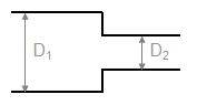
For ,
For ,
Tapered Reduction
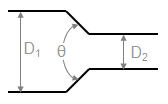
For , multiply from square reduction by a correction factor as follows:
For , multiply from square reduction by a correction factor as follows:
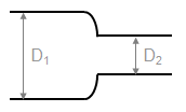
Rounded Pipe Reducer
Thin Sharp Orifice
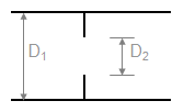
For ,
For
Thick Orifice
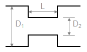
For , use the equations for a square reduction and a square expansion, otherwise multiply for a thin sharp orifice by a correction factor as follows:
Square Expansion
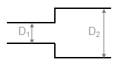
For
For
Tapered Expansion
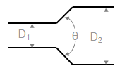
For use for a square expansion.
For multiply for a square expansion by:
Rounded Pipe Reducer (as expansion)
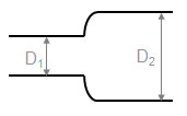
Use for square expansion.