Summary
Approximating a dataset using a polynomial equation is useful when conducting engineering calculations as it allows results to be quickly updated when inputs change without the need for manual lookup of the dataset. The most common method to generate a polynomial equation from a given data set is the least squares method. This article demonstrates how to generate a polynomial curve fit using the least squares method.
Definitions
| a | : | Polynomial coefficient |
| k | : | The degree of the polynomial |
| N | : | The number of points to be regressed |
| : | Error |
Introduction
When presented with a data set it is often desirable to express the relationship between variables in the form of an equation. The most common method of representation is a order polynomial which takes the form:
The above equation is often referred to as the general polynomial regression model with the error serving as a reminder that the polynomial will typically provide an estimate rather than an implicit value of the dataset for any given value of .
Polynomial Order
The maximum order of the polynomial is dictated by the number of data points used to generate it. For a set of data points, the maximum order of the polynomial is . However it is generally best practice to use as low of an order as possible to accurately represent your dataset as higher order polynomials while passing directly through each data point, can exhibit erratic behaviour between these points due to a phenomenon known as polynomial wiggle (demonstrated below).

Estimating the Polynomial Coefficients
The general polynomial regression model can be developed using the method of least squares. The method of least squares aims to minimise the variance between the values estimated from the polynomial and the expected values from the dataset.
The coefficients of the polynomial regression model may be determined by solving the following system of linear equations.
This system of equations is derived from the polynomial residual function (derivation may be seen in this Wolfram MathWorld article) and happens to be presented in the standard form , which can be solved using a variety of methods.
Solving for the Polynomial Coefficients
Cramer’s Rule
Cramer’s rule allows you to solve the linear system of equations to find the regression coefficients using the determinants of the square matrix . Each of the coefficients may be determined using the following equation:
Where is the matrix with the column replaced with the column vector (remembering the system is presented in the form ). For example could be calculated as follows:
Cramer’s rule is easily performed by hand or implemented as a program and is therefore ideal for solving linear systems. Additionally when solving linear systems by hand it is often faster than using row reduction or elimination of variables depending on the size of the system and the experience of the practitioner.
Example Application of Cramer's Rule
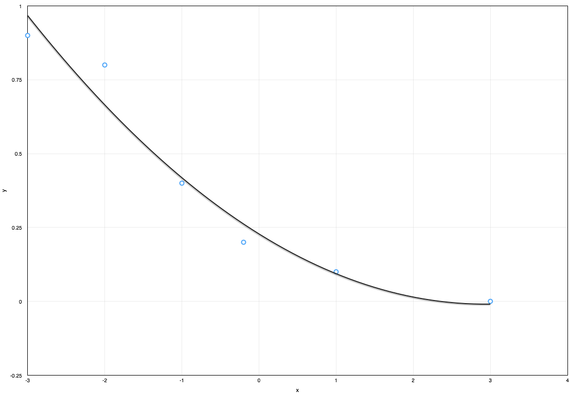
The following example demonstrates how to develop a 2nd order polynomial curve fit for the following dataset:
| x | -3 | -2 | -1 | -0.2 | 1 | 3 |
| y | 0.9 | 0.8 | 0.4 | 0.2 | 0.1 | 0 |
This dataset has points and for a 2nd order polynomial . As shown in the previous section, application of the least of squares method provides the following linear system.
Using Cramer’s rule to solve the system we generate each of the matrices by taking the matrix and substituting the column vector b into the ith column, for example and would be:
Once these matrices have been formed the determinant for each of the square matrices can be calculated and utilised to determine the polynomial coefficients as follows:
The polynomial regression of the dataset may now be formulated using these coefficients.
Which provides an adequate fit of the data as shown in the figure below.
LU Decomposition
LU decomposition is method of solving linear systems that is a modified form of Gaussian elimination that is particularly well suited to algorithmic treatment. Coverage of LU decomposition is outside the scope of this article but further information may be found in the references section below.
Software methods
There are several software packages that are capable of either solving the linear system to determine the polynomial coefficients or performing regression analysis directly on the dataset to develop a suitable polynomial equation:
- MATLAB
- A numerical computing environment commonly used in engineering.
- Mathematica
- A computational environment used in many industries.
- GNU Octave - An open source alternative to Matlab.
- R - A open source statistical computing package.
- Excel - A general purpose spread-sheeting program and an engineers primary tool
- Numbers - An alternative spread-sheeting program for Apple Mac and iOS platforms
It should be noted that with the exception of Excel and Numbers these packages can have a steep learning curve and for infrequent use it is more efficient to use Excel, Numbers or if solving manual Cramer’s rule.
References
Article Tags